Data from DINO
import matplotlib.pyplot as plt

import brodata
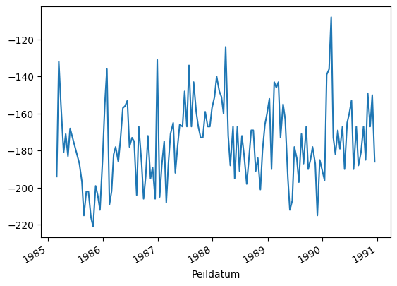
Groundwater heads
gws = brodata.dino.Grondwaterstand.from_dino_nr("B38B0207", 1)
gws
Grondwaterstand(Locatie='B38B0207', filter=np.int64(1), x=np.int64(117960), y=np.int64(439670))
gws.data
| Locatie | Filternummer | Peildatum | Stand (cm t.o.v. MP) | Stand (cm t.o.v. MV) | Stand (cm t.o.v NAP) | Bijzonderheid | Opmerking | |
|---|---|---|---|---|---|---|---|---|
| 0 | B38B0207 | 1 | 1985-02-28 | 177 | 107 | -194 | NaN | NaN |
| 1 | B38B0207 | 1 | 1985-03-14 | 115 | 45 | -132 | NaN | NaN |
| 2 | B38B0207 | 1 | 1985-03-28 | 138 | 68 | -155 | NaN | NaN |
| 3 | B38B0207 | 1 | 1985-04-15 | 164 | 94 | -181 | NaN | NaN |
| 4 | B38B0207 | 1 | 1985-04-29 | 154 | 84 | -171 | NaN | NaN |
| ... | ... | ... | ... | ... | ... | ... | ... | ... |
| 131 | B38B0207 | 1 | 1990-10-15 | 168 | 98 | -185 | NaN | NaN |
| 132 | B38B0207 | 1 | 1990-10-29 | 132 | 62 | -149 | NaN | NaN |
| 133 | B38B0207 | 1 | 1990-11-14 | 150 | 80 | -167 | NaN | NaN |
| 134 | B38B0207 | 1 | 1990-11-28 | 133 | 63 | -150 | NaN | NaN |
| 135 | B38B0207 | 1 | 1990-12-14 | 169 | 99 | -186 | NaN | NaN |
136 rows × 8 columns
gws.data.set_index("Peildatum")["Stand (cm t.o.v NAP)"].plot();
Groundwater quality
gwa = brodata.dino.Grondwatersamenstelling.from_dino_nr("B38B0079")
gwa
Grondwatersamenstelling(NITG-nr='B38B0079', x=118590, y=439850)
gwa.kwaliteit_gegevens_vloeibaar.T
| 0 | |
|---|---|
| NITG-nr | B38B0079 |
| Buis | 1 |
| Monster datum | 1959-06-22 00:00:00 |
| Monster-nr | C1959-06-1018 |
| Monster apparatuur | NaN |
| Mengmonster | nee |
| Bovenkant monster (cm tov MV) | 1400.0 |
| Onderkant monster (cm tov MV) | 3900.0 |
| Analyse datum | 1959-06-22 00:00:00 |
| CO2 (mg/l) | 12 |
| CO3 (mg/l) | 0 |
| Cl (mg/l) | 92 |
| EGV (uS/cm) | 57.6 |
| Fe (mg/l) | 2.6 |
| HCO3 (mg/l) | 207 |
| HH (mmol/l) | 2.538 |
| HHT (mmol/l) | 3.42 |
| Kleur (mgPt/l) | 19 |
| Mn (mg/l) | 0.96 |
| NH4 (mg/l) | 1.4 |
| NO2 (mg/l) | 0 |
| NO3 (mg/l) | 0 |
| NaHCO3 (mg/l) | 0 |
| PMV-ongf (mg/l) | 6 |
| PO4-tot (mg/l) | 0.46 |
| SO4 (mg/l) | 51.9 |
| T(5min)_veld (C) | 18 |
| pH (-) | 7.62 |
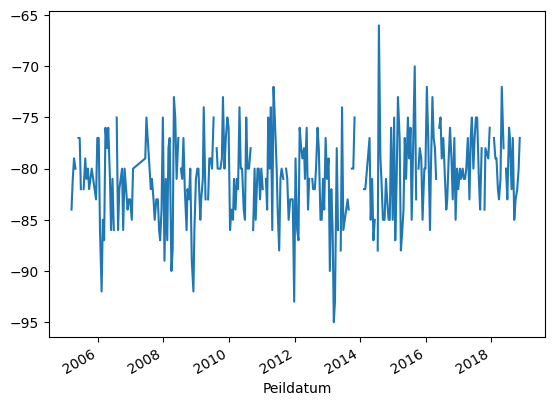
Surface water level
ows = brodata.dino.Oppervlaktewaterstand.from_dino_nr("P38G0010")
ows
Oppervlaktewaterstand(Locatie='P38G0010', x=np.int64(120502), y=np.int64(435210))
ows.data
| Locatie | Peildatum | Stand (cm t.o.v. NAP) | Stand (cm t.o.v. bovenkant Peilschaal) | Bijzonderheid | |
|---|---|---|---|---|---|
| 0 | P38G0010 | 2005-03-15 | -84.0 | 84.0 | NaN |
| 1 | P38G0010 | 2005-03-29 | -81.0 | 81.0 | NaN |
| 2 | P38G0010 | 2005-04-12 | -79.0 | 79.0 | NaN |
| 3 | P38G0010 | 2005-04-28 | -80.0 | 80.0 | NaN |
| 4 | P38G0010 | 2005-05-14 | NaN | NaN | NaN |
| ... | ... | ... | ... | ... | ... |
| 308 | P38G0010 | 2018-10-31 | -80.0 | 80.0 | NaN |
| 309 | P38G0010 | 2018-11-12 | -77.0 | 77.0 | NaN |
| 310 | P38G0010 | 2018-11-28 | NaN | NaN | NaN |
| 311 | P38G0010 | 2018-12-12 | -77.0 | 77.0 | NaN |
| 312 | P38G0010 | 2018-12-28 | NaN | NaN | NaN |
313 rows × 5 columns
ows.data.set_index("Peildatum")["Stand (cm t.o.v. NAP)"].plot();
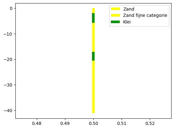
Drillings
gbo = brodata.dino.Boormonsterprofiel.from_dino_nr("B42E0199")
gbo
Boormonsterprofiel(NITG-nr='B42E0199', x=40815, y=414390)
gbo.lithologie_lagen
| Bovenkant laag (m beneden maaiveld) | Onderkant laag (m beneden maaiveld) | Kleur | Hoofdgrondsoort | Sublaag | Zandmediaan M63 | Zandmediaanklasse | Bijmenging kei | Lutum % | Bijmenging silt | Silt % | Bijmenging zand | Zand % | Bijmenging grind | Grind % | Bijmenging humus | Organische stof % | Kalkgehalte | |
|---|---|---|---|---|---|---|---|---|---|---|---|---|---|---|---|---|---|---|
| 0 | 0.0 | 0.3 | zwart | zand | NaN | NaN | NaN | NaN | NaN | NaN | NaN | NaN | NaN | NaN | NaN | NaN | NaN | NaN |
| 1 | 0.3 | 1.9 | onbekend | zand | NaN | NaN | fijne categorie (O) | NaN | NaN | NaN | NaN | NaN | NaN | NaN | NaN | NaN | NaN | NaN |
| 2 | 1.9 | 3.6 | onbekend | klei | NaN | NaN | NaN | NaN | NaN | NaN | NaN | NaN | NaN | NaN | NaN | humeus | NaN | NaN |
| 3 | 3.6 | 5.7 | onbekend | klei | NaN | NaN | NaN | NaN | NaN | NaN | NaN | NaN | NaN | NaN | NaN | humeus | NaN | NaN |
| 4 | 5.7 | 7.4 | onbekend | zand | NaN | NaN | fijne categorie (O) | NaN | NaN | NaN | NaN | NaN | NaN | NaN | NaN | NaN | NaN | NaN |
| 5 | 7.4 | 11.7 | onbekend | zand | NaN | NaN | fijne categorie (O) | NaN | NaN | NaN | NaN | NaN | NaN | NaN | NaN | NaN | NaN | NaN |
| 6 | 11.7 | 14.2 | onbekend | zand | NaN | NaN | fijne categorie (O) | NaN | NaN | zwak siltig | NaN | NaN | NaN | NaN | NaN | NaN | NaN | NaN |
| 7 | 14.2 | 15.7 | onbekend | zand | NaN | NaN | fijne categorie (O) | NaN | NaN | NaN | NaN | NaN | NaN | NaN | NaN | NaN | NaN | NaN |
| 8 | 15.7 | 17.1 | onbekend | zand | NaN | NaN | fijne categorie (O) | NaN | NaN | NaN | NaN | NaN | NaN | NaN | NaN | NaN | NaN | NaN |
| 9 | 17.1 | 20.5 | onbekend | klei | NaN | NaN | NaN | NaN | NaN | NaN | NaN | NaN | NaN | NaN | NaN | NaN | NaN | NaN |
| 10 | 20.5 | 26.5 | onbekend | zand | NaN | NaN | NaN | NaN | NaN | NaN | NaN | NaN | NaN | NaN | NaN | NaN | NaN | NaN |
| 11 | 26.5 | 29.8 | onbekend | zand | NaN | NaN | fijne categorie (O) | NaN | NaN | NaN | NaN | NaN | NaN | NaN | NaN | NaN | NaN | NaN |
| 12 | 29.8 | 33.5 | onbekend | zand | NaN | NaN | NaN | NaN | NaN | NaN | NaN | NaN | NaN | NaN | NaN | NaN | NaN | NaN |
| 13 | 33.5 | 36.9 | onbekend | zand | NaN | NaN | NaN | NaN | NaN | NaN | NaN | NaN | NaN | NaN | NaN | NaN | NaN | NaN |
| 14 | 36.9 | 37.6 | onbekend | zand | NaN | NaN | fijne categorie (O) | NaN | NaN | NaN | NaN | NaN | NaN | NaN | NaN | NaN | NaN | NaN |
| 15 | 37.6 | 41.2 | onbekend | zand | NaN | NaN | NaN | NaN | NaN | NaN | NaN | NaN | NaN | NaN | NaN | NaN | NaN | NaN |
f, ax = plt.subplots()
brodata.plot.dino_lithology(gbo.lithologie_lagen, ax=ax)
brodata.plot.add_lithology_legend(ax=ax);
Within extent
extent = [118000, 118400, 439560, 440100]
gdf = brodata.dino.get_boormonsterprofiel(extent)
gdf
| X-coordinaat | Y-coordinaat | CRS | Kaartblad | Bepaling locatie | Plaatsnaam | Provincie | Maaiveldhoogte (m tov NAP) | Bepaling maaiveldhoogte | Boormethode | Einddiepte (m beneden maaiveld) | Datum boring | Eigenaar | Uitvoerder | Organisatie Beschrijver | Beschrijvingsmethode | Nat/Droog beschreven | Kwaliteit beschrijving lithologie | lithologie_lagen | geometry | |
|---|---|---|---|---|---|---|---|---|---|---|---|---|---|---|---|---|---|---|---|---|
| NITG-nr | ||||||||||||||||||||
| B38B0160 | 118370 | 439630 | RD2000 | 38B | Onbekend | Schoonhoven | Zuid-Holland | 0.56 | Onbekend | NaN | 12 | 12-07-1958 | Onbekend | Visser en Smit, Papendrecht | Onbekend | Onbekend | Onbekend | E | Bovenkant laag (m beneden maaiveld) Onder... | POINT (118370 439630) |
| B38B0161 | 118390 | 439630 | RD2000 | 38B | Onbekend | Schoonhoven | Zuid-Holland | 0.56 | Onbekend | NaN | 15 | 10-07-1952 | Onbekend | Visser en Smit, Papendrecht | Onbekend | Onbekend | Onbekend | E | Bovenkant laag (m beneden maaiveld) Onderk... | POINT (118390 439630) |
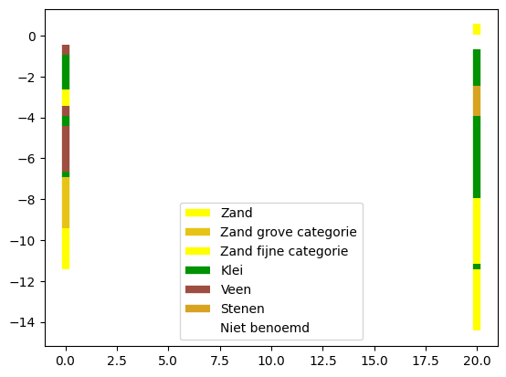
# plot the lithology along a line from west to east
y_mean = gdf.geometry.y.mean()
line = [(gdf.geometry.x.min(), y_mean), (gdf.geometry.x.max(), y_mean)]
brodata.plot.lithology_along_line(gdf, line, kind="dino");
Vertical electrical sounding
ves = brodata.dino.VerticaalElektrischSondeeronderzoek.from_dino_nr("W38B0022")
ves
VerticaalElektrischSondeeronderzoek(NITG-nr='W38B0022', x=119211, y=438265)
ves.data.T
| 0 | 1 | 2 | 3 | 4 | 5 | 6 | 7 | 8 | 9 | ... | 17 | 18 | 19 | 20 | 21 | 22 | 23 | 24 | 25 | 26 | |
|---|---|---|---|---|---|---|---|---|---|---|---|---|---|---|---|---|---|---|---|---|---|
| L/2 | 1.5 | 2.5 | 4.0 | 6.0 | 8.0 | 10.0 | 12.0 | 15.0 | 20.0 | 25.0 | ... | 125.0 | 150.0 | 175.0 | 200.0 | 250.0 | 300.0 | 350.0 | 400.0 | 500.0 | 600.0 |
| A | NaN | NaN | NaN | NaN | NaN | NaN | NaN | NaN | NaN | NaN | ... | NaN | NaN | NaN | NaN | NaN | NaN | NaN | NaN | NaN | NaN |
| V | NaN | NaN | NaN | NaN | NaN | NaN | NaN | NaN | NaN | NaN | ... | NaN | NaN | NaN | NaN | NaN | NaN | NaN | NaN | NaN | NaN |
| I | NaN | NaN | NaN | NaN | NaN | NaN | NaN | NaN | NaN | NaN | ... | NaN | NaN | NaN | NaN | NaN | NaN | NaN | NaN | NaN | NaN |
| R | 11.4 | 9.8 | 14.9 | 12.7 | 21.6 | 24.0 | 27.6 | 30.0 | 35.4 | 41.0 | ... | 51.0 | 48.0 | 52.0 | 49.8 | 46.9 | 42.1 | 34.8 | 30.8 | 21.7 | 17.1 |
5 rows × 27 columns
ves.data.set_index("L/2")["R"].plot(marker=".");
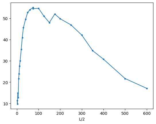
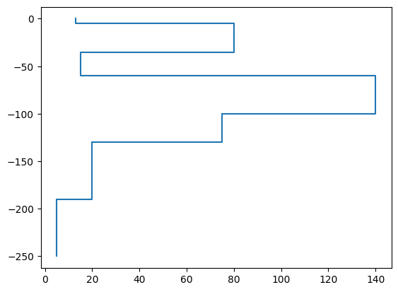
A vertical electrical sounding can have more than one interpretation; select the first interpretation.
ves.interpretaties[0]
| Bovenkant laag (m) | Onderkant laag (m) | Werkelijke weerstand | Lithologie | Grondwaterkwaliteit | Stratigrafische eenheid | |
|---|---|---|---|---|---|---|
| 0 | NaN | 4.5 | 13.0 | NaN | NaN | NaN |
| 1 | 4.5 | 35.0 | 80.0 | NaN | NaN | NaN |
| 2 | 35.0 | 60.0 | 15.0 | NaN | NaN | NaN |
| 3 | 60.0 | 100.0 | 140.0 | NaN | NaN | NaN |
| 4 | 100.0 | 130.0 | 75.0 | NaN | NaN | NaN |
| 5 | 130.0 | 190.0 | 20.0 | NaN | NaN | NaN |
| 6 | 190.0 | NaN | 5.0 | NaN | NaN | NaN |
We can also plot the resistivity of the interpretations. There is only one interpretation for this location, so we see only one line.
ves.plot_interpretaties();